Logo image

Coordinated Linear Algebra

Section 2.5 Matrix Transformations

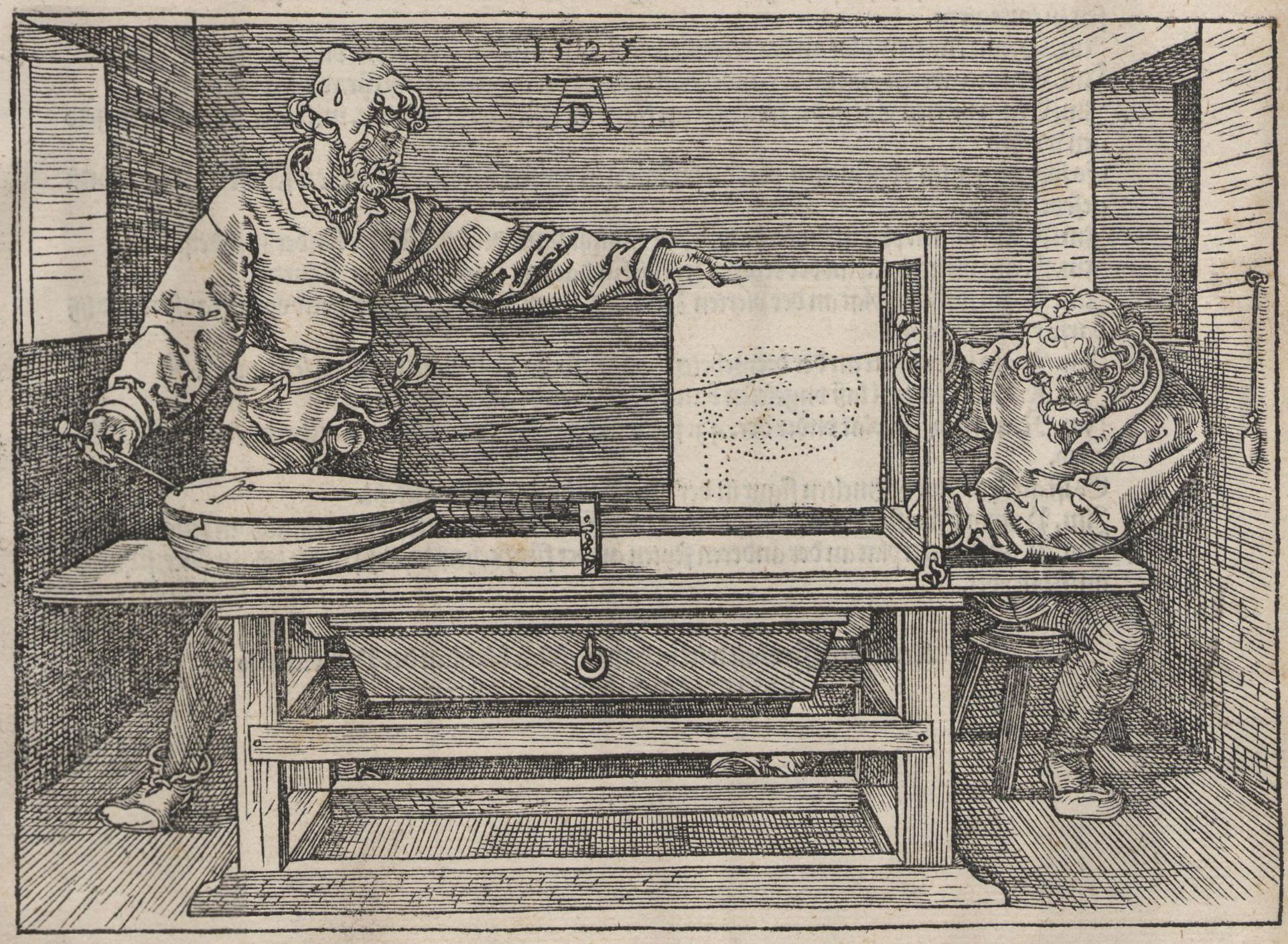
In the next two sections, we are going to look at matrices and matrix multiplication in terms of functions. Why would we do this? Well, consider the following woodcut, which is called The Draughtsman of the Lute and was made in 1525, about 500 years ago, by Albrecht Durer.
described in detail following the image
A lute is sitting on a table and a standing man is holding a string to part of the lute while a second man marks on a square frame where the string passes through the frame. Attached to the side of the frame is a square canvas which can be swung into the frame; marked on the canvas are various points that show the outline of part of the lute.
Figure 2.5.1. The Draughtsman of the Lute, Albrecht Durer, 1525
What are these two people doing? From our point of view, they are finding points in the three-dimensional space containing the lute, and then using the string and the wooden frame to work out the coordinates where the line of the string intersects the two-dimensional space of the frame. They then swing the picture back into the wooden frame and mark this point on the picture of the lute.
Long story short, they are building, point by point, a function from \(\R^3\) to \(\R^2\text{.}\)
People, or rather computers, still do similar calculations today. Every computer-animated film has similar functions to turn the three-dimensional models of the characters and setting into the two-dimensional frames of the film. It is natural for us to think of this as a function, whose domain is \(\R^3\) and whose codomain is \(\R^2\text{.}\)

Subsection 2.5.1 Functions from \(\R^n\) into \(\R^m\)

In the past you have worked with functions \(f:\R\longrightarrow \R\text{.}\) Most of the time such functions were defined algebraically. For example, we can define \(f\) by
\begin{equation*} f(x)=x^2. \end{equation*}
To fix our notation, we now define functions formally, along with some closely related terms.

Definition 2.5.2.

Let \(V\) and \(W\) be sets. A function \(f\) from \(V\) into \(W\text{,}\) denoted by
\begin{equation*} f:V\rightarrow W \end{equation*}
assigns to each element \(x\) of \(V\text{,}\) an element \(y=f(x)\) of \(W\text{.}\) Moreover, we use the the following terminology.
The set \(V\) is called the domain of \(f\text{,}\) and the set \(W\) is called the codomain.
If \(y=f(x)\text{,}\) we say that \(x\) maps to \(y\text{,}\) and \(y\) is the image of \(x\text{.}\)
Given some subset of \(V\text{,}\) call it \(X\text{,}\) we define the image of the subset \(X\) to be the set of \(f(x)\) for exactly those \(x\) in the subset \(X\text{.}\) The set \(f(V)\) is called the image or range of the function \(f\)
For our example function \(f(x)=x^2\) above, the domain and codomain are both \(\R\) and the image of the subset of real numbers less than -5 is the set of real numbers greater than 25. In symbols,
\begin{equation*} f(\{ x : x \lt -5 \}) = \{ y : y \gt 25 \}. \end{equation*}
Previously, you might have visualized function like \(f(x)=x^2\) by looking at its graph, the set of all points of the form \((x, f(x))\) in \(\R^2\text{.}\) In this course, we will find it more useful to look at functions diagrammatically. For instance, the diagram below shows that \(f\) maps 2 to 4. We say that 4 is the image of 2 under \(f\).
Function Domain and Codmain
We will now consider functions that map \(\R^n\) into \(\R^m\text{.}\) We will refer to such functions as transformations. There are two ways of thinking of transformations.
A transformation \(T:\R^n\longrightarrow\R^m\) can take a vector in \(\R^n\) and map it to a vector in \(\R^m\text{,}\) or it can map a point in \(\R^n\) to a point in \(\R^m\text{.}\) We think of transformations as acting on vectors or points interchangeably because every point
\begin{equation*} (x_1, x_2,\dots ,x_n) \ \text{ in} \R^n \end{equation*}
can be interpreted as the tip of a vector
\begin{equation*} [x_1, x_2, \ldots , x_n] \ \text{in } \R^n. \end{equation*}
Matrix multiplication will provide us with initial tools for defining some transformations.

Subsection 2.5.2 Examples of Matrix Transformations

Consider the matrix
\begin{equation*} A=\begin{bmatrix}1\amp 0.5\\0\amp 1\end{bmatrix}. \end{equation*}
The product of \(A\) with a \(2\times 1\) matrix (that is, a vector in \(\R^2\)) is again a \(2\times 1\) matrix. e can define a transformation \(T:\R^2\longrightarrow\R^2\) by \(T(\mathbf{x})=A\mathbf{x}\text{.}\) This transformation can be applied to every vector of \(\R^2\text{.}\) We will look at what it does to five vectors.
Vectors graphed
T and arrow drawn
T acted on vectors graphed
Even after looking at a handful of vectors it is often difficult to tell what the transformation actually accomplishes. This is why sometimes looking at points instead of vectors can be beneficial. If we consider every point in the left grid below as a tip of a vector, we can apply the transformation to each point to obtain the grid on the right.
Grid of points graphed
Applying \(T\) to a grid of points helps us see that the entire plane was sheared by the transformation.
We can also analyze the action of \(T\) algebraically. Start by finding the image of a generic vector \([x,y]\text{.}\)
\begin{equation*} T\left(\begin{bmatrix}x\\y\end{bmatrix}\right)=\begin{bmatrix}1\amp 0.5\\0\amp 1\end{bmatrix}\begin{bmatrix}x\\y\end{bmatrix}=\begin{bmatrix}x+0.5y\\y\end{bmatrix} \end{equation*}
We immediately see that the \(y\) component of the vector remains unchanged. We also see that the \(x\) component increases (or decreases) by an increment that depends on \(y\text{.}\) When considering \(T\) as a transformation acting on points, we see that points located 1 unit above the \(x\)-axis, get shifted to the right by 0.5. Points located 2 units above, get shifted to the right by 1. The higher the point, the greater the shift. Points with negative \(y\)-coordinates get shifted to the left. In this fashion \(T\) shears the entire plane.
Now that we have seen the effect of functions defined via matrix multiplication, we can better appreciate the term transformation, as such functions distort the domain and the shapes located in it. The following Exploration will help you visualize this.

Exploration 2.5.1.

Make your own shape by moving points \(A, B, C, D, E, F, G\) in the left pane. (You can also move the entire figure by clicking and dragging the whole polygon.) The images of the points and the polygon under the transformation induced by \(M\) are shown on the right.
Figure 2.5.3.
Try each of the following matrices to determine what each transformation accomplishes. (Type pi into GeoGebra to get \(\pi\text{.}\))
\begin{equation*} M_1=\begin{bmatrix}1\amp 0\\0\amp 2\end{bmatrix},\quad M_2=\begin{bmatrix}1/2\amp 0\\0\amp 1\end{bmatrix},\quad M_3=\begin{bmatrix}1\amp 2\\0\amp 1\end{bmatrix}, \end{equation*}
\begin{equation*} M_4=\begin{bmatrix}\cos(\pi)\amp -\sin(\pi)\\\sin(\pi)\amp \cos(\pi)\end{bmatrix},\quad M_5=\begin{bmatrix}\cos\left(\pi/4\right)\amp -\sin\left(\pi/4\right)\\\sin\left(\pi/4\right)\amp \cos\left(\pi/4\right)\end{bmatrix}, \end{equation*}
\begin{equation*} M_6=\begin{bmatrix}1\amp 0\\0\amp -1\end{bmatrix},\quad M_7=\begin{bmatrix}0\amp 1\\1\amp 0\end{bmatrix},\quad M_8=\begin{bmatrix}1\amp 1\\1\amp 1\end{bmatrix}. \end{equation*}
Problem 2.5.4.
Match each transformation below with the matrix \(M_1, M_2, \ldots , M_8 \) that induces it.
  1. Horizontal shear.
  2. Rotation by \(45^{\circ}\) counterclockwise.
  3. Reflection about the \(x\)-axis.
  4. Vertical Stretch.
  5. Maps everything to a straight line.
  6. Rotation through a \(180^{\circ}\) angle.
  7. Horizontal compression.
  8. Reflection about the line \(y=x\text{.}\)
Answer.
  1. \(\displaystyle M_3 \)
  2. \(\displaystyle M_5 \)
  3. \(\displaystyle M_6 \)
  4. \(\displaystyle M_1 \)
  5. \(\displaystyle M_8 \)
  6. \(\displaystyle M_4 \)
  7. \(\displaystyle M_2 \)
  8. \(\displaystyle M_7 \)
A \(2\times 2\) matrix induces a transformation from \(\R^2\) into \(\R^2\text{.}\) An \(m\times n\) matrix can be multiplied by an \(n\times 1\) matrix (that is, a vector in \(\R^n\)) on the right, with the resulting product being an \(m\times 1\) matrix. Therefore we can use an \(m\times n\) matrix \(A\) to define a transformation
\begin{equation*} T:\R^n\longrightarrow \R^m \ \text{ by } \ T(\mathbf{x})=A\mathbf{x}. \end{equation*}
We will call this transformation \(T\) a matrix transformation or, to be completely precise, the matrix transformation induced by \(A\). The example below showcases this concretely.

Example 2.5.5.

Let
\begin{equation*} A=\begin{bmatrix}1\amp 2\amp -1\\3\amp 2\amp -2\end{bmatrix}\text{.} \end{equation*}
Define a transformation \(T:\R^3\longrightarrow\R^2\) by \(T(\mathbf{x})=A\mathbf{x}\text{.}\) Find all vectors in the domain that map to \(\mathbf{0}\text{.}\)

Subsection 2.5.3 Linearity of Matrix Transformations

Recall the properties of matrix-vector multiplication from Remark 2.3.6,
\begin{equation} k(A\mathbf{v}) = A(k\mathbf{v})\tag{2.5.1} \end{equation}
\begin{equation} A(\mathbf{v}+\mathbf{w})= A\mathbf{v}+A\mathbf{w}\tag{2.5.2} \end{equation}
These two properties of matrix-vector multiplications give us corresponding properties of matrix transformations. Suppose \(T:\R^n\longrightarrow\R^m\) is a matrix transformation, then for all vectors \(\mathbf{v}\text{,}\) \(\mathbf{w}\) in \(\R^n\) and all constants \(k\) in \(\R\text{,}\)
\begin{equation} T(k\mathbf{v})=kT(\mathbf{v})\tag{2.5.3} \end{equation}
\begin{equation} T(\mathbf{v}+\mathbf{w})=T(\mathbf{v})+T(\mathbf{w})\tag{2.5.4} \end{equation}
In general, any transformation that satisfies (2.5.3) and (2.5.4) is called a linear transformation. As we have just seen, all matrix transformations are linear. We will study linear transformations more in the next section and revisit them throughout the text.

Subsection 2.5.4 Columns and the standard basis

In this section we will look at the images of standard unit vectors under a matrix transformation, and discuss why this information is helpful.

Exploration 2.5.2.

Let \(A=\begin{bmatrix}1\amp 2\amp 3\\4\amp 5\amp 6\\7\amp 8\amp 9\end{bmatrix}\text{.}\)
Problem 2.5.6.
Find the following products:
\begin{equation*} \begin{bmatrix}1\amp 2\amp 3\\4\amp 5\amp 6\\7\amp 8\amp 9\end{bmatrix}\begin{bmatrix}1\\0\\0\end{bmatrix}. \end{equation*}
\begin{equation*} \begin{bmatrix}1\amp 2\amp 3\\4\amp 5\amp 6\\7\amp 8\amp 9\end{bmatrix}\begin{bmatrix}0\\1\\0\end{bmatrix}. \end{equation*}
\begin{equation*} \begin{bmatrix}1\amp 2\amp 3\\4\amp 5\amp 6\\7\amp 8\amp 9\end{bmatrix}\begin{bmatrix}0\\0\\1\end{bmatrix}. \end{equation*}
Answer.
\begin{equation*} \begin{bmatrix}1\amp 2\amp 3\\4\amp 5\amp 6\\7\amp 8\amp 9\end{bmatrix}\begin{bmatrix}1\\0\\0\end{bmatrix}=\begin{bmatrix}1\\4\\7\end{bmatrix} \end{equation*}
\begin{equation*} \begin{bmatrix}1\amp 2\amp 3\\4\amp 5\amp 6\\7\amp 8\amp 9\end{bmatrix}\begin{bmatrix}0\\1\\0\end{bmatrix}=\begin{bmatrix}2\\5\\8\end{bmatrix} \end{equation*}
\begin{equation*} \begin{bmatrix}1\amp 2\amp 3\\4\amp 5\amp 6\\7\amp 8\amp 9\end{bmatrix}\begin{bmatrix}0\\0\\1\end{bmatrix}=\begin{bmatrix}3\\6\\9\end{bmatrix} \end{equation*}
Let \(T:\R^3\longrightarrow\R^3\) be a matrix transformation induced by \(A\text{,}\) then we can say that \(T\) maps \(\mathbf{i}\text{,}\) \(\mathbf{j}\) and \(\mathbf{k}\) to the first, second and third columns of \(A\text{,}\) respectively. This nice property is not limited to transformations induced by square matrices. Let \(T:\R^3\rightarrow \R^2\) be a linear transformation induced by
\begin{equation*} A=\begin{bmatrix}1\amp -2\amp 4\\0\amp 3\amp 5\end{bmatrix} \end{equation*}
Problem 2.5.7.
We will examine the effect of \(T\) on the standard unit vectors \(\mathbf{i}\text{,}\) \(\mathbf{j}\) and \(\mathbf{k}\text{.}\) Try and compute
\begin{equation*} T(\mathbf{i})=A\mathbf{i} \quad \text{and} \quad T(\mathbf{k})=A\mathbf{k}. \end{equation*}
Answer.
\begin{equation*} T(\mathbf{i})=A\mathbf{i}=\begin{bmatrix}1\\0\end{bmatrix},\quad T(\mathbf{j})=A\mathbf{j}=\begin{bmatrix}-2\\3\end{bmatrix}, \quad T(\mathbf{k})=A\mathbf{k}=\begin{bmatrix}4\\5\end{bmatrix} \end{equation*}
Observe that the image of \(\mathbf{i}\) is the first column of \(A\text{,}\) the image of \(\mathbf{j}\) is the second column of \(A\text{,}\) and the image of \(\mathbf{k}\) is the third column.
We formalize our findings in Exploration 2.5.2 as follows.

Observation 2.5.8.

In general, the linear transformation \(T:\R^n\rightarrow\R^m\text{,}\) induced by an \(m\times n\) matrix \(A\) maps the standard unit vectors \(\mathbf{e}_1\ldots \mathbf{e}_n\) to the columns of \(A\text{.}\) We summarize this observation by expressing columns of \(A\) as images of vectors \(\mathbf{e}_1\ldots \mathbf{e}_n\) under \(T\text{.}\)
\begin{equation*} A=\begin{bmatrix} a_{11} \amp a_{12}\amp \dots\amp a_{1n}\\ a_{21}\amp a_{22} \amp \dots \amp a_{2n}\\ \vdots \amp \vdots\amp \ddots \amp \vdots\\ a_{m1}\amp \dots \amp \dots \amp a_{mn} \end{bmatrix} = \begin{bmatrix} | \amp |\amp \amp |\\ T(\mathbf{e}_1) \amp T(\mathbf{e}_2)\amp \dots \amp T(\mathbf{e}_n)\\ |\amp | \amp \amp | \end{bmatrix} \end{equation*}
Why is it that knowing the images of standard unit vectors under a matrix transformation is helpful? Consider the following example.

Example 2.5.9.

Let \(T:\R^2\longrightarrow\R^2\) be a matrix transformation such that
\begin{equation*} T(\mathbf{i})=\begin{bmatrix}-2\\3\end{bmatrix} \ \text{ and } \ T(\mathbf{j})=\begin{bmatrix}1\\0\end{bmatrix}. \end{equation*}
Find \(T\left(\begin{bmatrix}-4\\10\end{bmatrix}\right)\text{.}\)
Now, Example 2.5.9 illustrates that a matrix transformation \(T:\R^n\longrightarrow\R^m\) is completely determined by where it maps the standard unit vectors. This is true because we can express every vector \(\mathbf{v}\) in \(\R^n\) as a linear combination of the standard unit vectors, then use (2.5.3) and (2.5.4) to find the image of \(\mathbf{v}\text{.}\)
Recall in Section 2.3 we defined the identity matrix \(I_n\) as the \(n\times n\) matrix whose \(j^{th}\) column is the standard unit vector \(\mathbf{e}_j\text{.}\) The identity matrix induces a matrix transformation \(T:\R^n\longrightarrow\R^n\) such that \(T(\mathbf{e}_j)=\mathbf{e}_j\) for all \(j=1,\ldots,n\text{.}\) This transformation maps every vector in \(\R^n\) to itself. For this reason, we call it the identity transformation.

Example 2.5.10.

Let \(T:\R^3\longrightarrow\R^3\) be the identity transformation, defined by \(T(\mathbf{x})=I_3\mathbf{x}\text{.}\) Find \(T\left(\begin{bmatrix}1\\2\\3\end{bmatrix}\right)\text{.}\)
Answer.
Observe:
\begin{align*} T\left(\begin{bmatrix}1\\2\\3\end{bmatrix}\right) \amp = \begin{bmatrix} 1\amp 0\amp 0\\ 0\amp 1\amp 0\\ 0\amp 0\amp 1 \end{bmatrix} \begin{bmatrix}1\\2\\3\end{bmatrix}\\ \amp = 1\begin{bmatrix}1\\0\\0\end{bmatrix} + 2\begin{bmatrix}0\\1\\0\end{bmatrix} + 3\begin{bmatrix}0\\0\\1\end{bmatrix}\\ \amp = \begin{bmatrix}1\\2\\3\end{bmatrix}. \end{align*}

Exercises 2.5.5 Exercises

1.

Let \(T:\R^2\longrightarrow \R^2\) be a matrix transformation induced by the matrix \(A\text{.}\) The GeoGebra window on the left shows the domain of \(T\text{,}\) with standard unit vectors \(\mathbf{i}\) and \(\mathbf{j}\text{,}\) and a vector \(\mathbf{x}\text{.}\) The window on the right shows the codomain of \(T\text{,}\) with the images of \(\mathbf{i}\text{,}\) \(\mathbf{j}\) and \(\mathbf{x}\) plotted.
Figure 2.5.11.
To use this interactive, you can
  • Change the entries of matrix \(A\text{;}\)
  • Change vector \(\mathbf{x}\) by dragging its tip.
Choose your matrix \(A\text{.}\) Visually verify the following claims:
  • The image of \(\mathbf{i}\) is the first column of matrix \(A\text{.}\)
  • The image of \(\mathbf{j}\) is the second column of matrix \(A\text{.}\)
Let \(\mathbf{x}=[2,1]\text{.}\) Complete the following statement by filling the blanks.
\begin{equation*} T(\mathbf{x})=T([\ ]\mathbf{i}+[\ ]\mathbf{j})=[\ ]T(\mathbf{i})+[\ ]T(\mathbf{j}) \end{equation*}
After having done that, change vector \(\mathbf{x}\) by dragging its tip. Observe the image of \(\mathbf{x}\) and its relationship to the images of \(\mathbf{i}\) and \(\mathbf{j}\text{.}\) Then fill the blanks below for a general vector \([a,b] \text{:}\)
\begin{equation*} T\left(\begin{bmatrix}a\\b\end{bmatrix}\right)=T([\ ]\mathbf{i}+[\ ]\mathbf{j})=[\ ]T(\mathbf{i})+[\ ]T(\mathbf{j}) \end{equation*}
Answer.
The expressions filled in are
\begin{equation*} T\left(\begin{bmatrix}a\\b\end{bmatrix}\right)=T(2\mathbf{i}+1\mathbf{j})=2T(\mathbf{i})+1T(\mathbf{j}), \end{equation*}
\begin{equation*} T\left(\begin{bmatrix}a\\b\end{bmatrix}\right)=T(a\mathbf{i}+b\mathbf{j})=aT(\mathbf{i})+bT(\mathbf{j}). \end{equation*}

2.

Show that a matrix transformation \(T:\mathbb{R}^{n}\rightarrow \mathbb{R}^{m}\) maps \(\mathbf{0}\) to \(\mathbf{0}\text{.}\) In other words, \(T\left(\mathbf{0}\right) = \mathbf{0}\text{.}\)

3.

Show that a matrix transformation \(T:\mathbb{R}^{n}\rightarrow \mathbb{R}^{m}\) maps a line in \(\R^n\) to a line (or the origin) in \(\R^m\text{.}\)
Hint.
A line in \(\R^n\) can be expressed as \(\mathbf{x}(t)=\mathbf{v}t+\mathbf{v}_0\text{.}\)